
RAG is a Data Engineering Heavy Problem: Building a Football ETL for AI
How to use a Pydantic airlock and a Golden Dataset to set the information right for your RAG

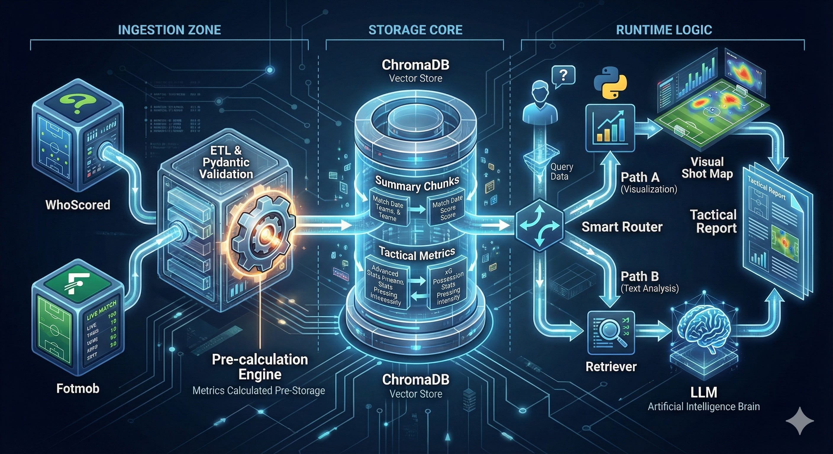
In my last post, I shared the big picture of the Football RAG system I’ve launched (Building a RAG System That Generates Football Post-Match Tactical Reports Automatically), and today, I want to talk about what is for me the most critical part of the system: the data pipeline.
RAG efficiency relies on great Data Engineering.
This refers to building a solid ETL process: Extract, Transform, Load — the process that prevents bad retrieval and bad generation, helping the system produce accurate responses.
So, I’ll go over the origin of the data, the sources I used, and the decisions I made to build the pipeline.
Where the Data Comes From
Starting from the main goal of the system: automatically provide concise post match reports using free updated post match data from a league gathered in one place. That way, you can save time hopping from one site to another and focus on what really matters: the analysis.
To build these tactical reports, I wanted to use match event data.
I reused and improved a version of the scrapers I built for my previous dashboard project. The goal was to move from scraping one match for a plot to indexing 108 matches for a system.
The main data sources are:
WhoScored: with more than 1,300+ events per match: passes, tackles, coordinates.
Fotmob: source for more specific match data like xG, numbers of shots and shot quality.
Fotmob provides the shot as a number, whereas WhoScored only provides if the action was a shot (True) or not (False). They complement each other.
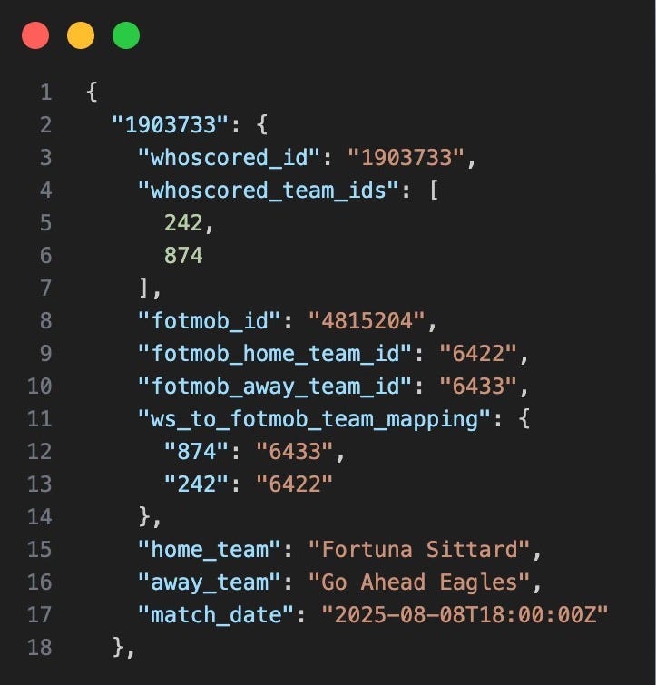
The first wall I hit in this Data Engineering process was: Entity Resolution.
Source A calls the team “R. Madrid,” Source B calls them “Real Madrid.” I needed to map them, so the RAG system wouldn’t think they are different teams.
Extracting the Data
The scrapers development evolved from a one-off scraping to more matches. In this case I used just 108 matches from the first leg of the Eredivisie league.
Why the Dutch league? It’s a league I’m really curious about, they are one of the best breeding talent leagues in Europe and it is always worth it looking at their emergent talents.
The scrapers followed a simple rule: the Raw information is immutable. I save the JSON exactly as it comes from the web into a “Raw Zone” (local for now). That way if I find a bug in my tactical metrics calculation later, I don’t need to scrape the web again. I just re-run it from the raw files.
Quick summary of how it works:
Scraper WhoScored --(JSON)--> [ Raw Zone /whoscored/ ]
                                            |
 Scraper Fotmob   --(JSON)--> [ Raw Zone /fotmob/   ]
                                            |
                              [ scrape_all_matches.py ]
                                            |
                               ( Orchestration & Logs )
The Workers: Specialized scrapers (one for WhoScored, another for Fotmob) designed with a single responsibility: extracting raw data.
The Storage: A local directory that serves as my immutable “Raw Zone.”
The Orchestrator: A central script (
scrape_all_matches.py) that acts as the conductor, identifying missing matches and triggering the workers accordingly.
# scripts/scrape_all_matches.py (A Simplified version of the Orchestrator)

def run_pipeline():
    # 1. Check what we already have (Incremental mode)
    existing_matches = get_local_raw_manifest()

    # 2. Run WhoScored Scraper
    print("🚀 Starting WhoScored extraction...")
    ws_data = scrape_whoscored_season(mode="incremental", exclude=existing_matches)
    save_to_raw_zone(ws_data, source="whoscored")

    # 3. Run Fotmob Scraper
    print("🚀 Starting Fotmob extraction...")
    fm_data = scrape_fotmob_eredivisie(mode="incremental", exclude=existing_matches)
    save_to_raw_zone(fm_data, source="fotmob")

    print("✅ Raw Zone updated. Ready for ETL.")
Pydantic Contracts: the “Airlock” Pattern
To safely store data in a vector database, I needed a Contract. It is a strict, machine-checkable definition of what your data must look like before it’s allowed to move downstream.
In my case, it’s the schema for a “valid match” (required fields, types, constraints). If the scraped payload doesn’t satisfy that contract—missing xG, null team IDs, wrong types—the pipeline fails fast and the match never gets stored in the vector database.
Pydantic is in charge to validate that match, working as an airlock. It defines exactly what a “valid match” looks like.

Pre-calculating +30 Metrics
Dumping 1,300 raw events into the LLM didn’t seem realistic nor cost-effective. It’s expensive in matters of tokens and slow latency, which ultimately confuses the model, making it prone to give back unreliable information.
Instead of the ETL just moving data, it acts as a Factory.
It processes raw, messy coordinates and distills them into Tactical Insights (or Actionable Metrics):
Instead of 500 raw pass coordinates → Verticality: 0.65
Instead of 20 defensive events → PPDA: 8.2
The logic is simple: I don’t want the LLM to waste its “brainpower” (and tokens) trying to do math on thousands of x,y points. I want it to focus on what it does best: reasoning over tactical concepts.
By pre-calculating these metrics, I’m handing the AI a “scout’s report” instead of raw notes.
This is the transformation step of the pipeline: where raw events, shots, and mappings are stitched together into a single, validated match profile.
# scripts/process_raw_data.py (simplified version of the transformation logic)

def process_matches():
    # 1. Load the "Glue": Match mappings and raw data
    mappings = load_json("data/match_mapping.json")

    for ws_id, mapping in mappings.items():
        # 2. Resolve IDs (The fix for the Home/Away swap bug)
        home_id, away_id = resolve_team_ids(mapping)

        # 3. Stitch data sources (WhoScored Events + Fotmob Shots)
        ws_data = load_json(f"raw/whoscored_matches/match_{ws_id}.json")
        fotmob_match = find_match_in_bulk(mapping['fotmob_id'])

        # 4. The "Factory": Distill 1,300+ events into 38 tactical metrics
        events_df = pd.DataFrame(ws_data['events'])
        raw_metrics = calculate_all_metrics(events_df, fotmob_match['shots'], home_id, away_id)

        # 5. The "Airlock": Validate everything with Pydantic
        match_profile = MatchProfile(
            metadata=MatchMetadata(match_id=ws_id, date=mapping['match_date']),
            home_team=TeamMatchStats(**map_metrics(raw_metrics, "home")),
            away_team=TeamMatchStats(**map_metrics(raw_metrics, "away")),
            home_score=calculate_score(fotmob_match['shots'], "home"),
            away_score=calculate_score(fotmob_match['shots'], "away")
        )

        # 6. Save to the Golden Dataset
        save_to_gold(match_profile)
In essence, it resolves team IDs, stitches two different data sources together, calculates tactical metrics, and finally passes everything through a Pydantic "airlock" to ensure the Golden Dataset is 100% reliable.
An issue I found at the beginning
Early in development, the system told me Zwolle dominated a game they actually lost 2-8 (https://www.sofascore.com/football/match/heracles-almelo-pec-zwolle/wjbsCjb)
The LLM was just reading the data I gave it and I thought it was hallucinating.
The ETL had a bug in the team ID mapping that swapped the Home and Away stats.
Something that made me understand that paying attention to the DE part is central.
The Golden Dataset & The Sniper Approach
The final output of the ETL is the matches_gold.json.
This file became the center of the system. Everything downstream: reports, evaluations, and rebuilds started here. That’s why I treat it as the Source of Truth, and not the vector database.
Once the data is in this shape, the next step was loading it into ChromaDB.
To do that, I used a simple 2-chunk architecture when indexing each match:
Summary Chunk: Contains match metadata: teams, date, score, and competition. Its job is to make sure the system finds the right match.
Tactical Chunk: Contains the pre-calculated metrics. This is what the LLM actually reads to generate the analysis.
I ended up calling this setup the “Sniper Approach.”
I wanted to avoid relying entirely on semantic search: embed the query, retrieve the closest vectors, and hope the correct match is somewhere near the top. That works, but it always felt a bit loose for this use case.
When a user asks about PSV vs Ajax, I don’t want the system to “kind of” get it right. I already know the exact match I’m looking for, so I use metadata filtering to narrow it down first. Once the match is identified, only then does the LLM see the tactical data.
This way, the vector database serves exactly what I ask for and retrieval becomes deterministic.
[SNIPPET F: scripts/rebuild_chromadb.py – Chunking & Metadata logic]
# scripts/rebuild_chromadb.py

for match in matches:
    match_id = match['metadata']['match_id']
    home = match['home_team']
    away = match['away_team']

    # Chunk 1: Summary (for metadata filtering)
    summary_text = (
        f"{home['team_name']} vs {away['team_name']} "
        f"({match['home_score']}-{match['away_score']}). "
        f"Possession: {home['possession']}% vs {away['possession']}%. "
        f"xG: {home['xg']} vs {away['xg']}."
    )

    summary_meta = {
        "match_id": match_id,
        "chunk_type": "summary",
        "home_team": home['team_name'],
        "away_team": away['team_name'],
        "match_date": match['metadata']['match_date']
    }

    collection.add(
        documents=[summary_text],
        metadatas=[summary_meta],
        ids=[f"{match_id}_summary"]
    )

    # Chunk 2: Tactical Metrics (for LLM generation)
    tactical_meta = {
        "match_id": match_id,
        "chunk_type": "tactical_metrics",
        "home_ppda": home['ppda'],
        "home_verticality": home['verticality'],
        "home_xg": home['xg'],
        "away_ppda": away['ppda'],
        "away_verticality": away['verticality'],
        "away_xg": away['xg'],
        # ... (38 total metrics)
    }

    collection.add(
        documents=[f"Tactical metrics for {home['team_name']} vs {away['team_name']}"],
        metadatas=[tactical_meta],
        ids=[f"{match_id}_tactical_metrics"]
    )
Two chunks per match: one for finding it (metadata filtering), one for analyzing it (LLM generation). The vector database doesn't guess; it serves exactly what I ask for.
I also added a sanitize_metadata() function to prevent ChromaDB from crashing on None values. It saved me from silent failures during indexing.
Link to the repo so you can check all the code: Football RAG Intelligence
Bottom Line
At the end of the day, a football analyst needs to trust the numbers, and a developer needs to trust the pipeline.
By building a strict ETL with Pydantic and a Golden Dataset, I managed to reduce the “hallucination surface” before even writing a prompt. The idea was to make the data so clear that the AI didn’t have to guess.
What’s next?
Now that we’ve tackled the data preparation, we need to talk to it.
In the next article, I’ll dive into the Prompt Engineering side of the project.
I’ll show you why I spent a good amount of time designing a Tailored Prompt and how that decision helped me cut token costs by 80%.
If you're interested in the intersection of Data Engineering and Generative AI, subscribe to follow this series.
See you then,
Ricardo.